.svg)

.svg)
Download Brouchure
%202.svg)
Oops! Something went wrong while submitting the form.
%201.svg)
Demand forecasting is the work of estimating future demand by taking historical sales and shipment data and layering in external variables such as seasonality and promotions. The resulting numbers flow into order quantities, safety stock, and production plans, and they serve as the baseline when multiple functions sit down to plan together. When the forecast wobbles, inventory costs and stockout risk rise together. This article walks through the definition of demand forecasting, its types, its methods and techniques, and the six steps of the process — and then follows the forecast all the way through to real ordering and inventory decisions.
In the meeting where next month's order quantity gets locked in, demand forecasting turns into a cost question immediately. Set it too high and unsold units pile up as warehouse carrying costs, then have to be cleared with markdowns once the season passes. Set it too low and your best-selling items run out first, with expedited procurement costs attached to every rushed refill.
Demand forecasting is the work of putting a number on how much will sell going forward. What that number actually describes, though, varies. It might be the growth direction of an entire market, or it might be how many units of a single SKU will move next week. What you forecast determines what data you need — and which teams end up consuming the output.

Demand forecasts and sales plans often come up in the same meeting, but they are fundamentally different things. A demand forecast is an estimate of what is likely to happen, built from the data collected so far and the variables already known. A sales plan adds targets and intent on top of that. It is a number that carries the ambition of how much the business wants to sell.
Collapsing the two into a single figure lets the target pull the forecast upward. When that inflated number flows straight into ordering, inventory piles up beyond what demand justifies. The better sequence is to lock the forecast first, then separate out the gap against the target and discuss it on its own terms.
Managing demand forecasting as its own discipline lets you look at inventory cost and stockout risk side by side, and it lets production, procurement, and finance plan against the same demand baseline.
Excess inventory shows up plainly on the books as carrying cost and tied-up capital, so it is easy to spot. Sales lost to stockouts are recorded nowhere, so they stay invisible. If the two losses are never compared side by side, the forecasting standard drifts toward whichever cost the books can see — and lost revenue from stockouts quietly drops out of the conversation.
Every function reads demand through a different lens. Sales looks at revenue targets; production looks at available capacity. Procurement starts with lead times, finance with cash flow. When each team walks into the meeting holding a different number, alignment takes longer, and every delayed decision eats into the slack available for procurement and production. A shared baseline converts the time spent reconciling numbers into time spent examining the reasoning behind them.
Forecasting demand in advance lets you set raw material contract timing, equipment utilization plans, and the amount of capital that will be tied up in inventory. For long lead-time items in particular, the forecast is what determines whether procurement happens at all. How far out the forecast horizon extends directly changes what volume you can actually secure.
When the baseline keeps shifting, production has to redo line assignments and shift plans. Procurement ends up backfilling long lead-time materials after the fact, and finance has to absorb inventory turnover and cash headroom drifting away from plan. Forecast quality is hard to judge on a single period's accuracy alone.
What you forecast, how far ahead you look, and how much anticipated change you build in all shape how a forecast gets used. Demand forecasting types can be sorted along five dimensions: application area, forecast horizon, forecasting approach, level of observation, and industry characteristics.
The phrase "demand forecasting" points at different objects — and different downstream decisions — depending on where it is used.
Search interest and marketing demand forecasting looks at when search volume for a given product category rises rather than at unit sales, and it is used to set campaign timing and budget.
In financial markets, demand forecasting refers to the book-building process of collecting and tallying institutional orders ahead of an issuance. For IPOs, bid prices and quantities determine the offering price; for corporate bonds, target rates and volumes determine the issuance rate. The term is the same, but the purpose has nothing to do with estimating future sales volume.
For business operations, product and operational demand forecasting is the one that matters. It analyzes product, SKU, channel, and promotion data together to estimate future sales volume, and that number goes straight into ordering and inventory decisions. Amazon Seller Central's product demand forecasting is another example of unit-level forecasts feeding replenishment decisions.
Each horizon connects to a different class of decision. The longer your order lead time, the further out you need to look — so the horizon has to match the decision cycle of the work if the forecast is going to get used at all.
Passive demand forecasting assumes that past sales patterns will largely continue, and simply extends the historical trend forward. It suits companies with steady revenue and a product mix that does not change often. It also requires relatively little data, which keeps preparation simple.
Active demand forecasting adds anticipated future changes into the mix — new channel launches, major promotions, product introductions, and other factors that have not yet appeared in historical data. It fits companies in a growth phase or with a frequently shifting sales structure. Without a clear rule about who adds which variables and on what evidence, though, the forecast can tilt toward the target number.
Macro-level forecasting looks at movement across an industry or category and feeds investment and business planning. Micro-level forecasting works at narrower units — a specific channel, customer segment, or individual SKU — and feeds ordering and allocation.
Demand forecasting estimates how much the market or customers will actually buy or order, and how much will be sold or shipped. Those estimates then become key inputs to the operations plans built downstream.
Forecasts by SKU or distribution channel, for instance, get converted into labor hours, production lines, and warehouse or transport units, and from there into calculations of how much capacity, equipment load, staffing, and logistics throughput will be required. Those calculations are then compared against the resources actually available to decide production schedules, shift patterns, outsourcing, and how inventory will be run.
The forecasting target shifts by industry even within product and operational demand. In manufacturing and distribution, finished goods and component shipment volumes and channel-level SKU sales drive production volume, ordering, and store allocation. In F&B, where shelf life is short, and in fashion, where products sell on a seasonal cycle, the questions that surface are days of supply, initial order quantity, and when to trigger markdowns.
Demand forecasting methods fall into three families: qualitative methods, statistical and time-series methods, and AI and machine learning methods. Time-series data here means data that accumulates in chronological order, such as daily sales volume or weekly shipments.
Qualitative methods rest on human judgment. They are used when there is no historical data, or when the data that exists cannot explain what comes next.
The Delphi method polls a panel of experts anonymously, shares the results back, and collects opinions again over several rounds. The design exists to avoid the situation where the loudest voice in the room drives the conclusion. It suits new technologies or new markets with no sales curve to reference. The repeated rounds do take time.
In the sales force composite method, field representatives submit expected sales for their accounts and those figures are aggregated into an overall forecast. It brings in information that never makes it into a system — the mood at an account, a deal in progress that has not been logged. When quota pressure is high, the numbers can skew in one direction, so the estimates need to be corrected against the gap between past submissions and actual sales.
Market research and surveys ask about purchase intent directly and are used to gauge early demand ahead of a product launch. Because stated intent and actual purchase diverge, the emphasis should be on relative preference ordering rather than absolute unit numbers.
Expert judgment and panel consensus bring merchandising, marketing, and sales together to adjust the forecast in one sitting. Reconciling multiple perspectives at once produces a fast conclusion. Without a written record of the reasoning, though, it becomes hard to know what to fix in the next cycle.
Statistical techniques find the regularity inside a historical sales curve and extend it forward. The calculation is transparent, which makes it easy to explain why a number came out the way it did.
Moving averages use the average of the last several periods as the forecast for the next one. Weighted moving averages put more weight on recent periods, so they react a little faster to change. The simplicity makes them a common choice for building a baseline. For items with a strong trend or heavy seasonality, though, they always lag a beat behind.
Exponential smoothing weights recent data heavily while retaining a diminishing share of older values. Simple exponential smoothing handles level only, Holt's method adds trend, and Holt-Winters adds seasonality as well. It performs reliably on items whose seasonal patterns repeat consistently year to year.
ARIMA uses both past values and past errors to estimate the next value. It performs well when data is plentiful and the pattern is regular, but each item needs its own parameter tuning, which becomes labor-intensive as the SKU count grows.
Regression and econometric models explain sales volume through other variables such as price, advertising spend, weather, or economic indicators. They let you quantify how sales move when price drops by a given amount. The catch is that you need future values for the explanatory variables before you can use them.
Seasonal indices express how much more an item sells in a given month or week relative to normal, then multiply that index into the forecast. They are a straightforward way to capture demand tied to fixed dates such as holidays or a summer peak.
AI techniques learn across many items and many variables at once, surfacing patterns no person could track simultaneously.
Boosting-family models train on sales history together with variables such as price, promotions, day of week, weather, and stock position. They perform reliably on tabular operational data, which is why they are widely used in practice. They also show how much each variable contributed to the forecast.
Deep learning time-series models are strong on complex structures — relationships between distant time points, or the influence items exert on one another. Data volume and training cost rise alongside that capability, so it is worth confirming item count and history length before deciding where to apply them.
Hierarchical forecasting handles demand across nested layers — total, category, SKU — and reconciles them so the sums line up at every level. Training many items together also lets a new product with thin history borrow the pattern of a similar product family.
In practice, stable items and volatile ones, items with deep history and brand-new products all sit in the same portfolio. No single method covers all of them. The more reliable approach is to segment by item group and assign methods accordingly — qualitative judgment for new products with no history, statistical techniques for regular items, machine learning for large assortments tangled up with promotions.
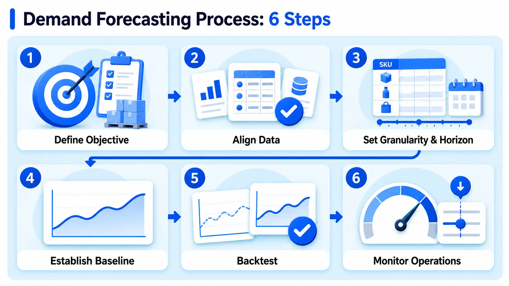
Demand forecasting runs through six steps: defining the forecast objective, verifying data consistency, setting the forecast unit and horizon, establishing a baseline, selecting and backtesting a model, and monitoring in operation. The improvement you gain from clarifying objectives and data standards in the early steps is generally larger than what you gain from swapping models in the later ones. Skipping ahead is rarely worth it.
Forecast accuracy should be assessed with MAPE, WAPE, and Bias together. Look at any one of them alone and the same forecast can be judged two different ways.
Even with a healthy MAPE, if Bias runs consistently in one direction on your highest-volume items, inventory cost keeps leaking while the headline number looks fine. There is no absolute threshold at which a given metric is "good enough." What works better is tracking whether error direction is improving against prior forecasts, item group by item group. Metric calculations and how to read them are covered in more depth in our guide to demand forecast error and accuracy metrics.
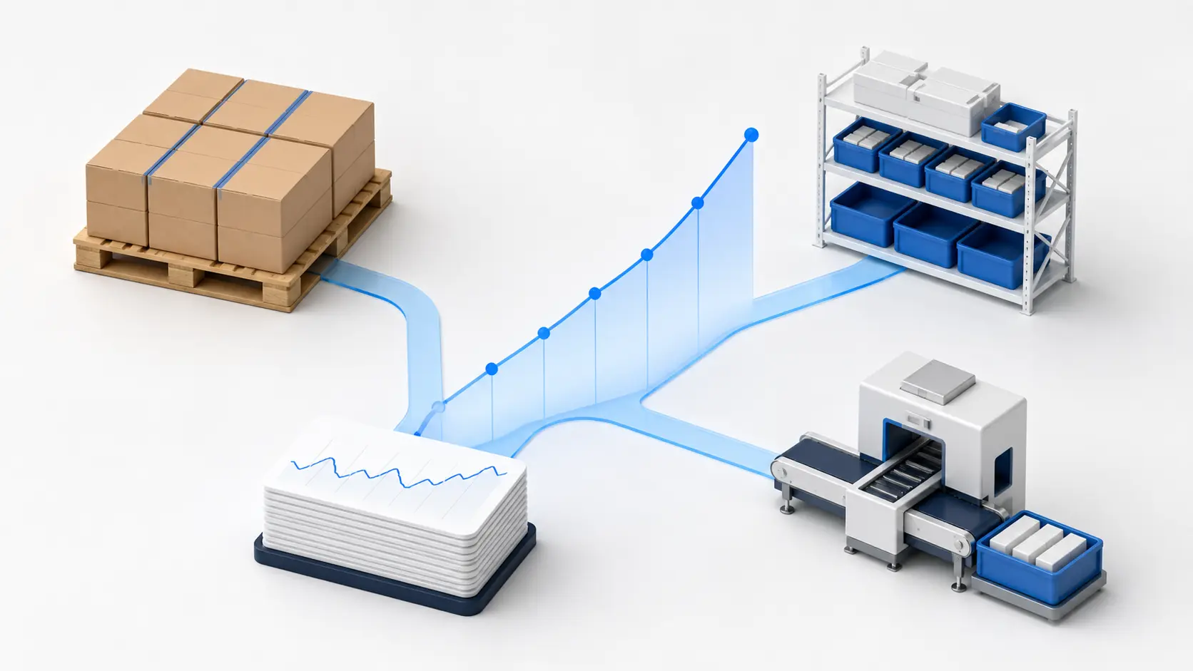
Eliminating forecast error entirely is not possible. What matters is the direction the error runs and how often it occurs. That error ultimately shapes how much safety stock you hold and how order quantities get set, and it shows up directly in your inventory position.
Safety stock is the buffer held against the forecast missing. It grows thicker as demand volatility rises, as lead times lengthen, and as the target service level goes up. Cycle service level refers to the probability of getting through a single replenishment cycle without a stockout; 95% means aiming to clear roughly 95 out of 100 replenishment cycles without running out.
The same magnitude of error carries a different price on an item where stockouts are expensive than on one where carrying cost dominates. Apply a single service level to everything and one group sits permanently exposed to stockout risk while the other sits permanently exposed to excess inventory.
A point forecast offers a single number — "demand next month will be around 1,000 units." A 90% prediction interval instead says something like "demand next month is expected to fall between 900 and 1,150 units," showing the range the outcome is likely to land in. The interval is constructed so that, across repeated forecasts, actual demand falls inside it roughly 90% of the time.
Deciding orders from a point forecast alone leaves no room for how much actual demand could vary. With a prediction interval, you can compare scenarios at the lower bound, midpoint, and upper bound, which gives you firmer footing for safety stock, production, and logistics planning.
The buyer takes forecast demand, subtracts current inventory and inbound receipts, then sets the order quantity with safety stock and lead time factored in. The production planner uses that same forecast to set output volume and equipment utilization plans. A baseline that does not keep getting overturned matters as much as the accuracy of any single number.
Promotions and new products share one problem: the answer is not inside the normal sales curve.
Promotional demand requires looking beyond regular sales history to the promotion type, duration, and discount depth. Promotions and price cuts are variables that deliberately disturb demand, so a model trained only on normal sales patterns explains neither the spike during the discount window nor the drop-off after it ends. The more that past promotions' sales volume, post-promotion decline, and channel-level response are captured in data, the better the model reflects them.
For new products, early demand is estimated by linking the item to past products with similar fabrication, category, price point, and seasonality, and reading the sell-through velocity of that product family. There is no prior-year SKU to compare against, which rules out a year-over-year approach for early demand. Placing a similar product's curve alongside it helps distinguish whether the response right after launch is a short-lived exposure effect or a genuine demand signal. Looking only at aggregate totals hides the skew where popular colorways or sizes sell out first. Demand has to be broken out by channel and SKU to be manageable at the unit where ordering and allocation actually happen.

S&OP — sales and operations planning — is the meeting where sales, production, procurement, and finance sit down around a single AI-generated demand baseline and align ordering and production plans against it.
To build the baseline, AI combines internal sales and shipment data with external variables such as promotions, weather, and economic indicators, and trains across many SKUs and channels at once. In effect, it applies a consistent standard to multi-item patterns no person could monitor simultaneously. McKinsey notes that applying AI forecasting to the supply chain can reduce forecasting error by 20 to 50%, though that figure is a reference point that varies considerably by industry, data, and operating conditions. AI also struggles to read ahead on events that reach the data late — a sudden weather shift, a competitor's major campaign, a supply delay. That is why a step where people adjust the exception items identified earlier has to sit alongside it.
Every function reads the same demand against a different standard. Rather than letting each team interpret the forecast on its own, S&OP puts what each one looks at and what each one decides in the same room.
Because the perspectives differ this much, alignment slows down when the meeting becomes an exercise in defending each team's own number. Lock the reference forecast first, then compare scenarios — the upper and lower bounds of the prediction interval, and a supply delay case — and finalize ordering and production plans from there. After execution, review where and by how much the forecast missed, and feed that back into the next baseline. Run the loop a few times and the meeting time spent reconciling numbers shrinks. Meeting structure and the monthly operating rhythm are laid out in our AI demand forecasting and S&OP process guide.
Decide who owns the forecast and who may adjust it before rollout, and decide where the reasoning behind adjustments gets recorded. Leave that undefined and decisions revert to the old way even as the forecast improves.
As item and channel counts grow, generating forecasts, isolating anomalous items, and assembling the reasoning to present in meetings all repeat every cycle. When that repetition outgrows what one person's time can absorb, forecasting operations tooling comes into the conversation.
Deepflow, from ImpactiveAI, is an AI solution that supports SKU-level demand forecasting and inventory decision-making.
Deepflow presents forecasts alongside the external variables that influenced them and each variable's contribution. When evaluating a tool, accuracy is only half the question — the other half is whether the person responsible can explain in a meeting why the number came out the way it did.
Items projected to run short or long can be viewed as a list in the BI dashboard, which cuts the time it takes to isolate the exception items defined earlier. When procurement, production, logistics, and sales all look at at-risk inventory on the same screen, aligning judgment gets easier. LLM-based analysis reports summarize forecasts and trends in narrative form, ready to use as cross-functional briefing material.
In the S&OP meeting, teams review Deepflow's forecast data and at-risk item lists against the scenarios discussed earlier, and use them as reference in adjusting ordering, inventory, and production plans. Final decisions on order quantities and inventory levels remain with the practitioners and meeting participants; Deepflow's role is to organize and supply the forecast evidence and the items that need review.
Forecasting models are built by standardizing customer data, combining it with external environmental data, and then selecting from over 224 candidate models the one that fits that company's data. The statistical and machine learning techniques described above both sit inside that candidate pool, so different methods get selected depending on the character of the item group. ImpactiveAI continues to advance its demand forecasting and commodity price forecasting technology on the basis of 80 patents. Commodity price forecasting is the adjacent track that companies looking to extend forecasting into purchase timing decisions typically evaluate alongside it.
Forecasting performance depends on data quality, product characteristics, operating processes, and how well external variables are captured, so quantified impact is calculated during the data diagnostic stage using your own data. Among documented customer cases, Ildong Foodis — an F&B company that has to manage stockouts and overstock together because of shelf-life constraints — reduced inventory risk by more than 26%.
Whether you are ready comes down to whether you can answer the questions below — before you start picking models. If several are hard to answer, the right sequence is to sort out data and workflows first.
Set gates by deciding in advance what has to be confirmed at each evaluation stage before moving to the next.
Timeline and cost vary with data condition, integration scope, and the number of item groups, so it is safer to settle those during the requirements definition stage.
It is the work of estimating future demand by adding external variables such as seasonality and promotions to historical sales and shipment data. Because the resulting numbers flow into order quantities, safety stock, and production plans, what decision the forecast serves matters as much as the forecast itself.
In business operations, product and operational demand forecasting — which handles sales volume at the product and SKU level — is the central type. Market and customer demand forecasting, and financial market demand forecasting for IPOs or corporate bonds, serve entirely different purposes. By horizon, forecasts split into short term for ordering, medium term for S&OP, and long term for investment decisions.
Passive forecasting extends past sales patterns forward as they are. Active forecasting builds in anticipated changes such as new channels or major promotions. The more frequently a company's sales structure shifts, the better active forecasting fits — but it needs a defined process for justifying which variables get included.
They fall into qualitative methods such as expert judgment, Delphi, and sales force composite; statistical and time-series methods such as moving average, exponential smoothing, ARIMA, and regression; and AI and machine learning methods including boosting and deep learning families. Since history and volatility differ item by item, methods are assigned by item group.
Use qualitative methods for new products or new markets with no sales history to reference. Quantitative methods fit established items with sufficient history. In practice, the common pattern is to build the baseline quantitatively and then adjust only the exception items with qualitative judgment.
Six: defining the forecast objective, verifying data consistency, setting the forecast unit and horizon, establishing a baseline, selecting and backtesting a model, and monitoring in operation. Following the sequence means you still have a basis for comparison when you swap models later.
Sales and shipment history organized by SKU, channel, and date is the foundation. Adding inventory, price, and promotion history lets the model capture drivers of variation as well. When coding schemes differ across systems, consistency verification is the first task.
It fits manufacturing, distribution, F&B, and fashion companies with enough SKUs and channels that generating forecasts and assembling the reasoning behind them is no longer practical to repeat manually. It suits organizations aiming to bring ordering, inventory, and S&OP decisions onto a single forecast standard.
Forecasting demand perfectly is not a realistic goal. Knowing the direction of your error and setting safety stock and service levels differently by item group keeps the cost of being wrong inside a manageable range. Before choosing types and methods, the things to settle are what you are forecasting, how far ahead, and which decision — ordering, production, or S&OP — the number will serve. Working through the checklist questions and the evaluation-stage table above will show you how far your current data and decision processes actually are.
If you want to know how far your own data can take you, get in touch with ImpactiveAI. We can run a PoC on your data to establish forecast accuracy first. If you include your managed SKU count, the length of your sales and shipment history, how ordering and S&OP currently run, and the inventory problem weighing on you most, we can ground the very first conversation in your own numbers.
.svg)

.svg)

.svg)









%201.svg)
%202.svg)


