Why Do Raw-Material Price Changes Reach Purchase Costs at Different Speeds?

For teams buyin

If a cost outlook simply says, “copper is up, soybeans are up, and naphtha is up,” it is almost certain to invite follow-up questions. Even when all three markets move in the same direction on the same day, the impact on an actual purchase price can arrive at very different times.

That gap is not simply a matter of market volatility. It comes from the way each commodity is priced, contracted, shipped, and consumed.

‍

Three Variables That Determine Pass-Through Timing

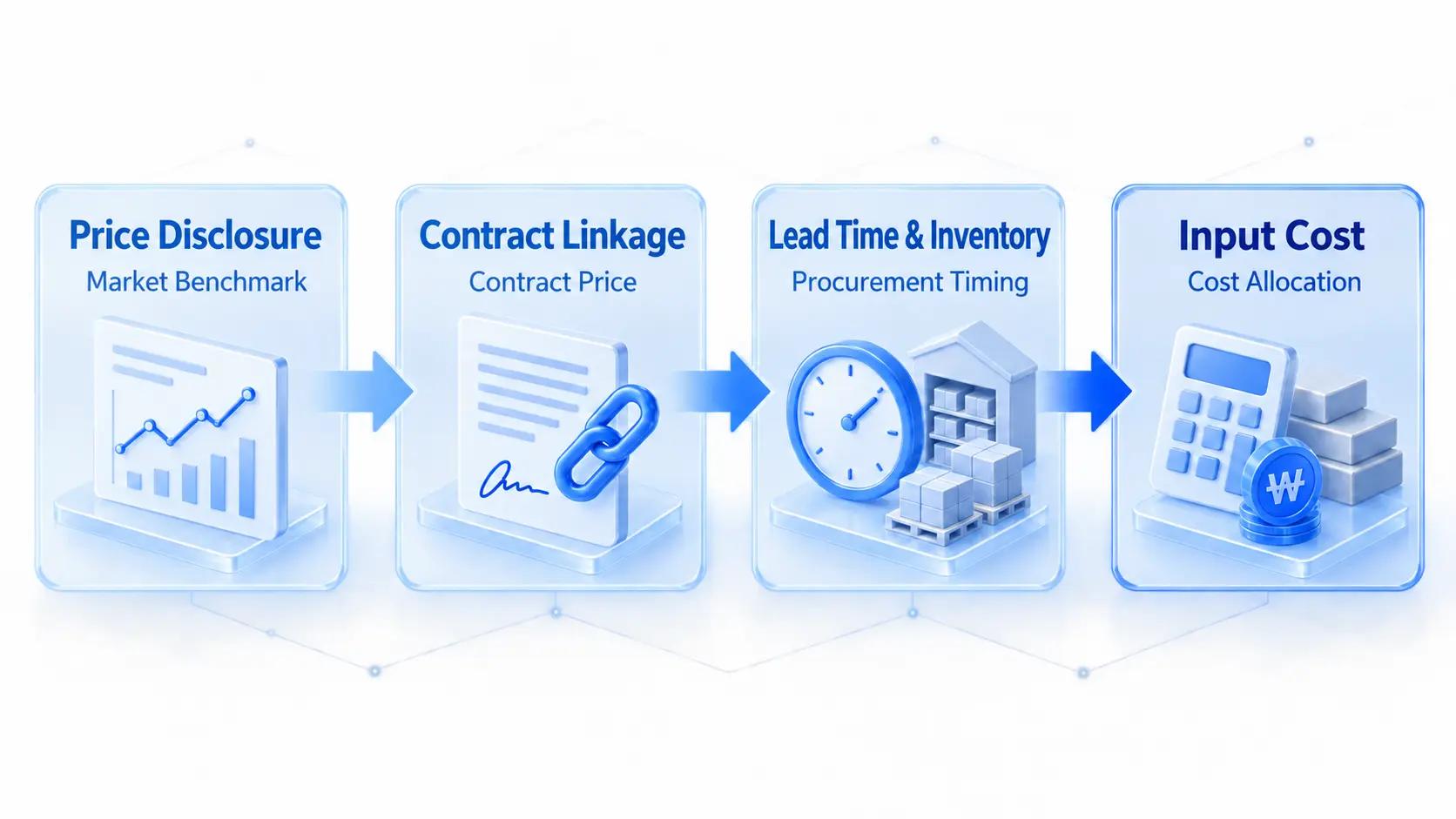
The first question is where a price is published and how often it is updated. For commodities with a daily exchange close, the gap between the market reference price and the contract price can be very small. Where a price is index-linked or negotiated quarterly, however, market movements and purchase prices are naturally further apart.

The second variable is the contractual rule for incorporating that market price. In non-ferrous metals contracts, the Quotational Period (QP) specifies the period used to set the price. Choosing the average for the shipment month rather than the arrival month can shift the purchase price by roughly a month, even when the underlying market trend is unchanged. For products purchased at a fixed quarterly price, the unit price remains unchanged throughout the contract term, and accumulated movements are reflected all at once at renewal.

The final variable is lead time and inventory. A company importing grain by bulk vessel is likely using feedstock today that was priced several months earlier. If the warehouse holds two months of inventory, today’s market price may not affect production cost until two months from now.

‍

Metals: Pricing Months and Settlement Mechanics

Copper and Nickel

When a daily reference price is published, an actual procurement contract generally adds a premium based on region and product form to arrive at the final price. When the market rises, that movement tends to flow through to later settlement with little delay. The levers available to the buyer are usually limited to the premium level, volume allocation, the QP, and the timing of price fixing.

Iron Ore and Coking Coal

Index-linked pricing has become standard for these materials, shortening the lag compared with the past. But the materials still move through steelmaking before steel products are priced again with downstream customers. As a result, a buyer of finished steel may not feel a change in raw-material prices immediately.

Scrap is different. Steelmakers often publish their purchase prices directly, and those prices can take effect quickly. Domestic supply-demand conditions, however, can cause the local scrap market to diverge from international benchmarks.

For teams buying metal raw materials, the key operational issue is often the decision deadline. It is easy to lose a favorable pricing window while checking the market and moving through internal approval. A sound market view is not enough if the pricing period closes before a decision is made.

‍

Agricultural Commodities: Import Lead Times and Cost Lags

Futures prices for globally traded agricultural commodities such as soybeans and corn can move sharply several times in a day. The landed cost faced by a buyer, however, is not determined by futures alone. Basis, ocean freight, foreign exchange, and customs-clearance costs are added in sequence before the final delivered cost is known.

Import lead time is just as important. Even if Chicago futures jump today, the effect on a company’s actual input cost usually arrives three to six months later. Prices can also rise briefly on crop concerns and retreat once the harvest outcome becomes clear. A forward-buying decision based solely on a short-term price spike can therefore lock in unexpectedly expensive inventory.

For dairy ingredients such as cheese, supply contracts are often set on a quarterly or semiannual basis. Even when the market falls, the contracted price remains in force until the next renewal, at which point the adjustment is made in one step. When forecasting agricultural input costs, it is often more useful to review contracted volume remaining and inbound shipment schedules than to watch the spot chart alone.

‍

Petrochemicals: Stage-by-Stage Lags and Pass-Through Rates

Timing gaps emerge at every stage of the petrochemical supply chain: from crude-oil refining upstream, to naphtha, base chemicals such as ethylene and propylene, resins such as PE and PP, and finally converted products downstream.

An even more important variable is the spread between the feedstock and the finished product. Resin prices are shaped not only by feedstock cost, but also by operating rates and the global supply-demand balance. When supply is ample, producers often absorb part of a naphtha increase. When supply is tight, prices may rise by the full increase in feedstock cost—or more. That is why petrochemical procurement requires more than an assessment of pass-through timing. Buyers also need to assess how much of an input-cost increase is actually being passed on.

For a company buying packaging or converted plastic products, the effect takes longer still to become visible. A supplier’s price-increase notice may arrive months after an oil-price headline. To judge whether that increase is justified, the buyer needs a clear record of how prices changed at each stage in between.

How Pass-Through Timing Differs by Commodity Group

‍

The final column can be used directly in a procurement meeting. For metals, the question is the decision deadline. For agricultural commodities, it is when committed supply and inventory will run out. For petrochemicals, it is whether a supplier’s requested increase is justified.

‍

The Data Behind a Procurement Decision

Knowing the timing characteristics of a commodity does not, by itself, decide whether to buy ahead, stagger purchases, or wait. That decision still requires judgment. In practice, market prices and FX are often checked in separate systems, while supplier quotations are compared with prior prices through a new spreadsheet every month.

To make the calculation properly, external data—market prices, FX, and freight—must be connected with internal purchase history, contract prices, and supplier quotations. The model also needs to account for real operating constraints such as lead time, minimum order quantities, inventory, and carrying costs. External market data alone produces a market commentary. Add internal procurement data, and the team can calculate savings in the context of its own business.

‍

Deepflow Materials Forecasting: From Market Signals to Purchase Decisions

Calculating these timing differences manually every month is difficult. The timing of pass-through differs not only across commodities, but also across the drivers of a single commodity: FX, inventory, and indicators from downstream industries can each affect price on a different schedule.

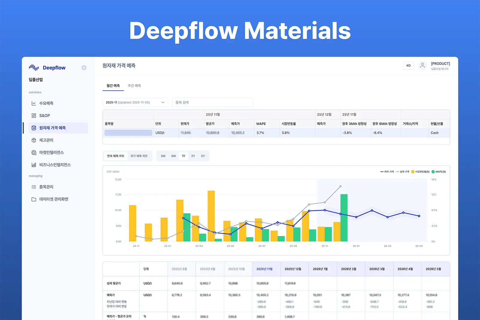
This is the complexity a forecasting model must address. In a rebar price forecasting project that Impactive AI conducted with a construction company, forecast performance improved not by adding variables indiscriminately, but by aligning each indicator with the period in which it actually affects price. The model treated inputs differently: the two-month change in FX, the four-month trend in construction starts, and the one-month inventory-to-sales ratio for rebar each had their own lag and transformation. The resulting model achieved an average forecasting accuracy of 95.59% in the project.

The same variables and lags will not apply identically to every market, of course. Each commodity requires its own model design.

What the procurement team sees is the result of that analysis: an outlook for the coming months, the direction of travel, predicted versus actual values, and error metrics in one place. Rather than recalculating every individual lag, the team can use the forecast to decide whether to buy now or wait.

The underlying drivers of a price movement are also documented, which makes the output useful as evidence in internal reporting. Deepflow does not place purchase orders on the buyer’s behalf. The buyer still decides what to buy, when to buy it, and in what quantity. Deepflow reduces the time spent gathering data and working through spreadsheets, so procurement professionals can focus on the decisions that matter.

If you would like to see the price outlook and forecast performance for a material you manage, apply for a Deepflow Materials demo. You can evaluate one forecasted commodity directly for one to two weeks.

‍