Download Brouchure

Oops! Something went wrong while submitting the form.

MAPE, or mean absolute percentage error, is the most widely used metric for evaluating demand forecast error. It tells you how far your forecasts missed actual demand, on average, in percentage terms. That makes it easy to compare items with very different sales volumes on the same footing.
In this article, we'll start with how to calculate MAPE and interpret the result. From there, we'll look at how to handle periods where actual demand is zero, and how MAPE differs from MAE, RMSE, WMAPE, and sMAPE. We'll wrap up with Excel formulas you can drop straight into your own workbook.
MAPE takes the error in each period, divides it by the actual value to get the absolute percentage error (APE), and then averages those APEs and expresses the result as a percentage.
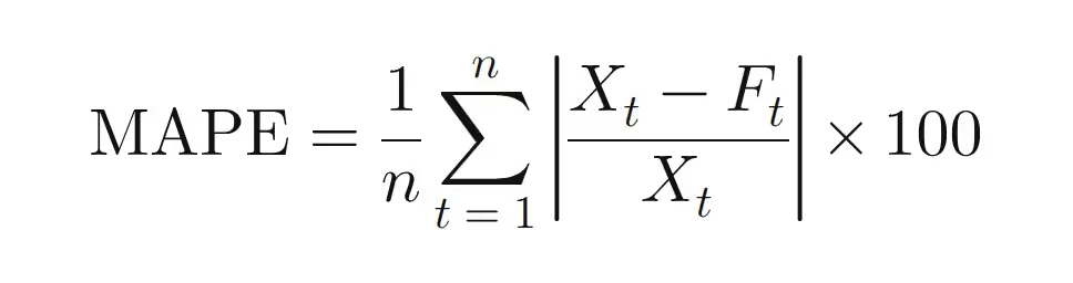
Here, Xt is actual demand in period t, Ft is the forecast, and n is the number of data points. Taking the absolute value strips out the direction of the error, so only its magnitude is measured relative to actuals.
Suppose a product's actuals and forecasts over three months look like this.
Add up the three monthly APEs and divide by three, and you get a MAPE of roughly 14.4%.
A MAPE of 14.4% means the forecast missed actual sales by about 14.4% per month on average. In practice, many teams subtract MAPE from 100% and call the result (85.6% here) "forecast accuracy." Keep in mind that this is a convention, not a rigorous accuracy metric, so if you use it as a KPI for decision-making, document exactly how it's defined.
Looking month by month, February, the lowest-volume month, posted an APE of 25.0% and pulled the overall average up considerably. February's absolute error of 20 units was double that of the other months, and because actual sales were also lower, the percentage error widened even further. When your data includes low-volume months or items like this, MAPE can come out higher than the error you actually feel on the ground. That's why it pays to check APE by month or by item when interpreting the result.
Because actuals sit in the denominator, MAPE simply can't be calculated for any period with zero sales. Add a no-sales period to the earlier data, say April with an actual of 0 and a forecast of 5, and here's how the results change by metric.
WMAPE (weighted mean absolute percentage error) doesn't simply average the period-level error rates. Instead, it divides the sum of absolute errors by the sum of actual sales.
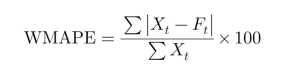
Because the denominator is total sales, the calculation still works even when some periods have zero actuals. It also gives more weight to errors in high-volume periods, which makes it a good fit when you want to assess forecast performance in unit terms. Two caveats apply, though. It can't be calculated if total actual sales are zero, and errors on low-volume items can get masked by high-volume items.
Each metric looks at error from a different angle, so practitioners typically use two or more together depending on the goal. The table below applies each metric to the January–March example and lays out where each one fits best.
The accuracy metrics above only show the magnitude of error. To see whether your forecasts lean consistently in one direction, you need to look at MPE (mean percentage error) separately. Because MPE doesn't take the absolute value, over-forecasts show up as positive values and under-forecasts as negative ones, and the two offset each other. In this article, MPE is calculated as the average of (forecast − actual) ÷ actual. Some sources use (actual − forecast) instead, so confirm the sign convention before comparing numbers.
Applying this definition to the earlier example gives +2.2%, meaning forecasts ran slightly high overall. Persistent positive bias can lead to inventory build-up, while persistent negative bias raises stockout risk. That's why it's good practice to monitor a bias metric that shows the direction of error alongside your accuracy metrics.
A report stating "MAE of 500 units" only makes sense if you know total sales volume, but "MAPE of 5%" immediately tells you the forecast was off by about 5% on average. That makes it easy for non-technical stakeholders to grasp, and it serves as a common language when departments set accuracy targets. The ability to compare items with very different sales volumes on the same percentage scale is another big reason it's so popular in practice.
There are, however, a few things to watch for when interpreting MAPE. First, when actuals are zero or very small, the result can be heavily distorted. For an item that sells only one or two units, even a small miss can push the error rate into the hundreds of percent. For slow-moving or intermittent-demand items like these, MAPE alone isn't a reliable basis for judgment.
Second, the error rates for over-forecasting and under-forecasting are asymmetric. If actual demand is 100 and you forecast 0, the error rate tops out at 100%. Forecast 500, and it climbs to 400%. As a result, focusing solely on minimizing MAPE can bias a model toward forecasting below actual demand. In categories where stockouts are especially costly, such as fresh food or essential medicines, it's best to read MAPE together with other metrics, including bias.
There's no hard-and-fast threshold for a good MAPE. That said, the interpretation scale from Lewis (1982) is widely cited and often used as a reference range. Because the appropriate level varies by industry, aggregation level, and forecast horizon, no single number works as a universal pass mark.
What's actually achievable depends on the sector, the item, and how accuracy is measured.

Rather than anchoring to external benchmarks, it's more realistic to use your own historical forecast performance as the baseline. For example, calculate the MAPE of a naive forecast that simply carries last month's actuals forward as next month's forecast. That shows you how much your current forecasting method actually improves on the baseline. For a fair comparison, measure performance on a holdout set that mirrors your real forecast origin and horizon, not on the data the model was trained on.
It's best to set targets separately for each product group. For low-volume groups, consider rolling them up and managing them with WMAPE at the product-group level.
If you're just getting started with forecast error tracking, Excel alone is enough to build a basic framework.
Assuming columns A through D hold date, SKU, actual (column C), and forecast (column D), with data starting in row 2, you can use the following formulas.
Format the result cells as percentages. Because aggregate bias is calculated from total error, it can differ from MPE, which averages period-level percentages.
Use a pivot table to roll up results by product group and by planner, and apply conditional formatting to flag items that exceed your threshold so you can spot them at a glance. Placing MAPE and WMAPE side by side makes it easy to tell when MAPE is inflated purely by low-volume items.
Once you're managing hundreds or thousands of SKUs and need to factor in external drivers like weather and promotions, the time spent calculating metrics item by item and diagnosing the root causes of error grows dramatically. ImpactiveAI's Deepflow is an AI demand forecasting SaaS built for practitioners at exactly this stage.
Deepflow automatically selects the best-fit model for each SKU's sales pattern from a library of more than 224 machine learning and deep learning models, and generates forecasts backed by 75 patented technologies. Because steady core items and erratic sellers get different models, planners no longer have to tune the forecasting approach item by item.
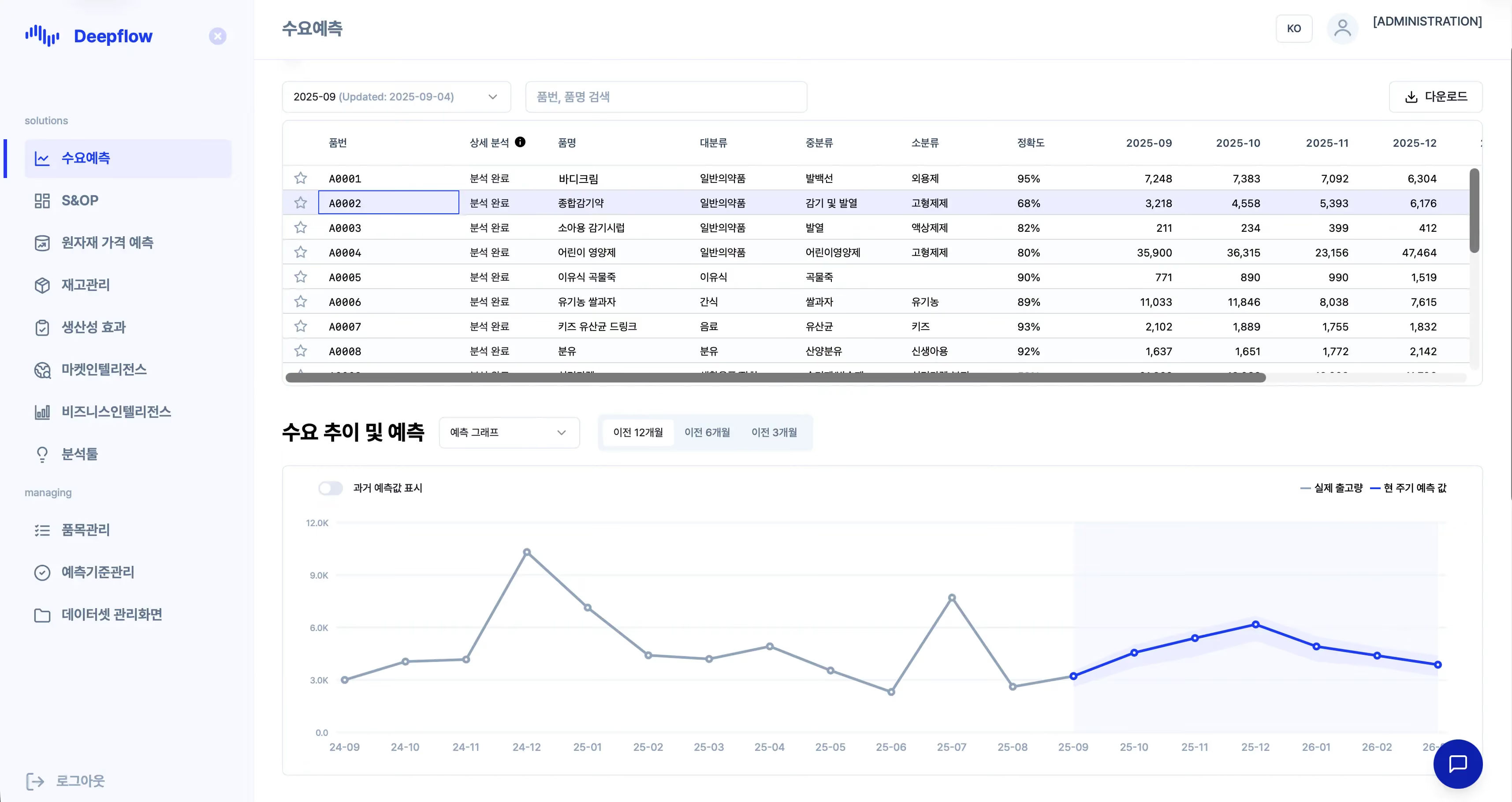
An error rate on its own doesn't tell you what to change. Deepflow's LLM-powered analytical reports automatically summarize historical sales trends, the rationale behind each forecast, and department-specific action plans. Sales, production, and procurement can work from the same forecast rationale to discuss their own responses, cutting the time spent diagnosing error and building reports. Ildong Foodis, for example, reduced its inventory risk by more than 26% after adopting Deepflow.
Forecast error management starts with using MAPE to understand where you stand today. Layer in WMAPE and bias metrics from there, then evaluate an AI solution once SKU counts and external drivers grow, and you'll have a framework where the whole organization works from the same numbers. Curious what forecasts your own sales data would produce? See for yourself with a Deepflow PoC.
MAPE is a simple average of period-level error rates, while WMAPE divides total absolute error by total sales. WMAPE gives more weight to errors in high-volume periods and can still be calculated when some periods have zero actuals.
Yes. If the forecast is more than double the actual, the error rate for that period exceeds 100%. There's no upper bound on error in the over-forecasting direction.
In practice, forecast accuracy is commonly defined as 100% minus MAPE, so a MAPE of 14.4% translates to 85.6% accuracy. Because this is a conventional conversion, it turns negative once MAPE exceeds 100%. When you report it, note which metric it was derived from.
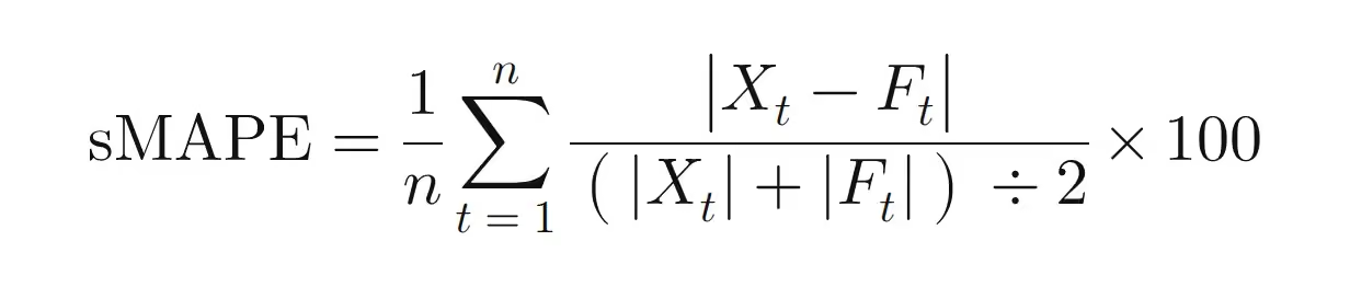
sMAPE is a relative error that uses the average of the actual and the forecast as its denominator, and its defining feature is that results are bounded between 0% and 200%. Despite the name, it isn't truly symmetric. For errors of the same size, under-forecasts yield a higher value. With an actual of 100, a forecast of 90 gives about 10.5%, while a forecast of 110 gives about 9.5%. It also returns 200% when the actual is zero and the forecast isn't, and it's undefined when both are zero, which makes it hard to use as a standalone metric for items that rarely sell.
For intermittent-demand items with frequent zero-sales periods, percentage-based metrics alone won't give you a reliable picture. A common alternative is MASE (mean absolute scaled error), which expresses your forecast's error as a multiple of the mean absolute error of a naive forecast that carries forward the previous period's actual (Hyndman & Koehler, 2006). A MASE below 1 means your average error is smaller than that baseline's. Pair it with operational metrics like stockout rate and excess inventory to see whether forecast error is actually turning into cost.