What Do AI Demand Forecasting Models Learn? From Sales Patterns to Time Lags Between Variables

Even when the same product is sold at the same price, sales volumes vary from day to day. They depend on whether it is a weekend, whether a promotion is running, and which channel the product appears on. This is why sales from the same month last year and recent averages alone are insufficient to estimate next month’s demand.

How do AI demand forecasting models capture these differences? They begin by learning from data. They identify not only trends and seasonality in historical sales, but also how demand has varied with conditions such as price, promotions, weather, and sales channels, then estimate demand under new conditions.

When evaluating a model, it is therefore essential to examine both the algorithm it uses and the inputs and relationships it is designed to learn. Even the same algorithm can produce different results depending on how variables are constructed and aligned in time.

‍

The Fundamentals of AI Model Training: Linking Sales Conditions to Outcomes

To forecast weekly sales, input data can include each historical week’s prices, promotion status, product attributes, and recent sales trends. The model uses these inputs to generate predictions, compares them with actual sales, and adjusts its internal computational rules to reduce prediction errors.

Once training is complete, the model estimates next week’s sales using the information available for that forecast. However, explaining historical results well is different from accurately forecasting demand for an unseen period. Performance must be evaluated on subsequent periods excluded from training to assess the model’s practical value.

The first step is to define the forecasting target. Sales volumes, shipment volumes, and actual customer demand are not always the same. Without accounting for sales lost during stockouts or shipments that customers purchase in advance, the model may learn supply constraints or advance purchasing as characteristics of demand.

Before deciding which data to include, establish what those numbers actually represent.

‍

What Demand Forecasting Models Learn: Trends, Seasonality, and Variability

The patterns AI learns do not imply that the same quantity will sell on the same date every year. Rather, the model identifies relationships that recur across different periods and conditions, even when individual sales figures vary.

Typical examples include trends, such as steady sales growth, and seasonality, where demand concentrates in certain seasons or on particular days of the week. Models can also examine relationships between variables involving price or promotional conditions, variability in sales volumes, and anomalous patterns that deviate from typical behavior.

Two products may have the same average sales volume, yet one sells consistently each week while the other experiences periods with no orders followed by large order spikes. This distinction matters for ordering and inventory management. However, not every model automatically learns all these characteristics. Addressing irregular orders and demand uncertainty requires appropriate data and model design.

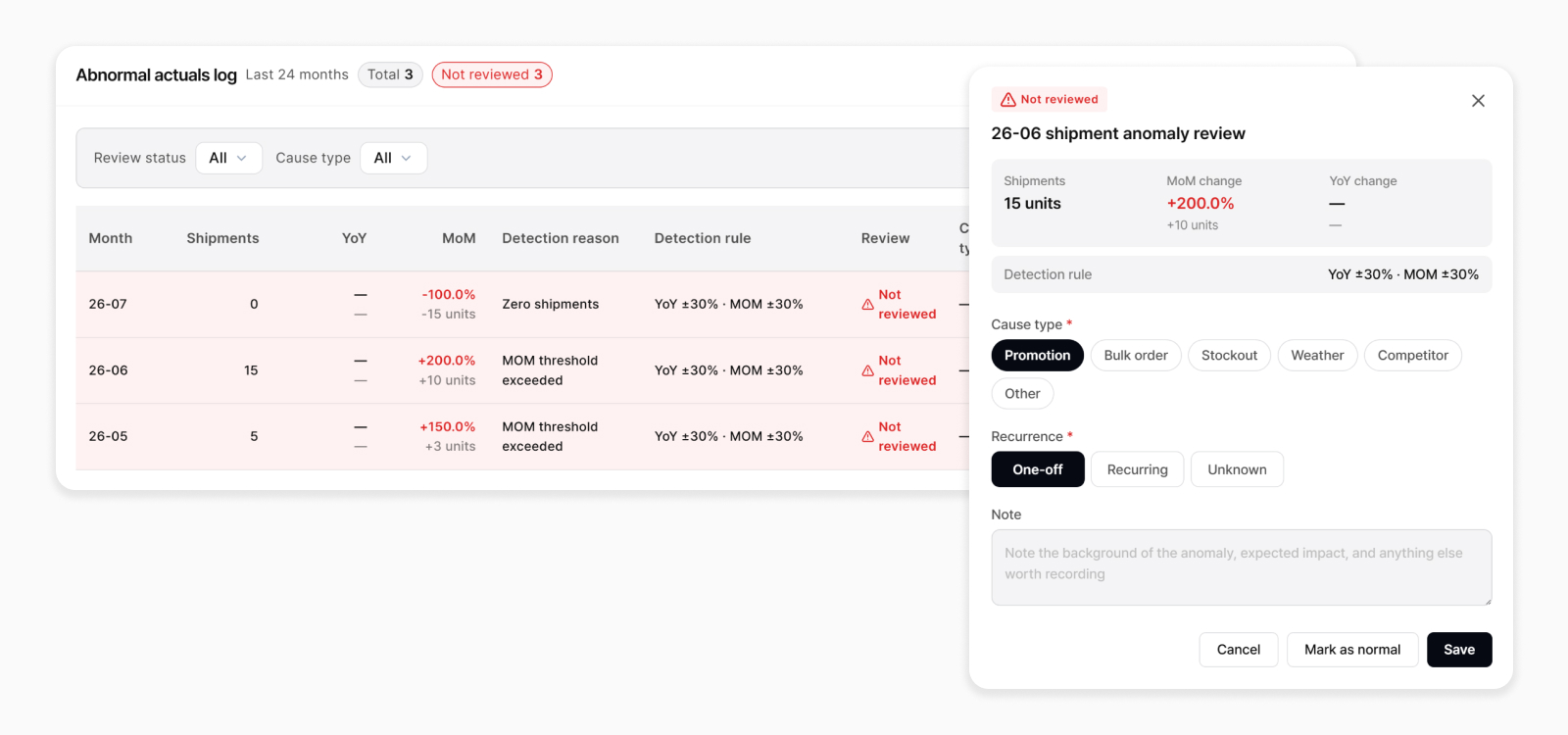
A sudden sales increase should not automatically be treated as noise to remove. It may reflect a real response to a promotion or external exposure. Identifying and recording the cause provides useful context when similar conditions arise again.

‍

Nonlinear Relationships and Interactions Among Discounts, Weather, and Channels

Doubling the discount rate does not necessarily double the increase in sales. Small discounts may generate little response until a threshold is reached, or deeper discounts may produce almost no additional sales. This is known as a nonlinear relationship.

Multiple conditions can also act together. The same discount may generate different responses on an off-season weekday and a peak-season weekend. This is called an interaction: the effect of a discount changes depending on other conditions.

Machine learning models for demand forecasting can be designed to learn these relationships. Rather than simply concluding that discounts increase sales, they analyze which discount conditions were associated with changes in sales for particular products and channels.

For this reason, aligning price, weather, and promotion data with the same products and periods is just as important as collecting those variables. If promotion schedules are recorded weekly but sales are recorded daily, the data must be aligned with the actual promotion dates and conditions.

‍

Distinguishing Time Lags in External Variables from Causality

Purchases do not all occur on the day search activity increases. Customers may research a product and buy it several days later. In manufacturing, changes in activity within customer industries may also take time to translate into actual orders.

A time lag can therefore exist between a change in a variable and a change in the forecasting target. Indicators from one or two months earlier may be more useful for explaining this month’s demand than indicators from the current month.

The timing of variables was also important in a rebar price forecasting project Impactive AI conducted for a construction company. The project gathered a wide range of data, including exchange rates, interest rates, floor area of construction starts, permitted building floor area, rebar production, and inventories. However, adding more variables or applying more complex models alone delivered limited performance improvements.

This was because each indicator was reflected in prices at a different point in time. Indicators related to construction plans may be associated with changes that emerge after relatively long lags, while the inventory-to-sales ratio may reflect more immediate supply and demand conditions. Comparing all variables using only values from the same month makes it difficult to capture these timing differences adequately.

Impactive AI analyzed which historical time points provided useful predictive information for each variable. Based on the findings, it constructed variables with different lags and transformations, such as the exchange rate’s rate of change two months earlier, the trend in floor area of construction starts four months earlier, and the rebar inventory-to-sales ratio one month earlier. The model incorporating this lag structure achieved an average forecasting accuracy of 95.59% in the project.

This result reflects the evaluation criteria used in that project; the same variables and lags will not apply to every market. It nevertheless demonstrates that improving forecasting performance requires designing not only which data to collect, but also which historical values to use and how to represent them for training.

Of course, preceding an outcome does not establish causality. Even if search activity rises before sales increase, both changes may be driven by advertising. Time-lagged relationships that are useful for prediction must be distinguished from causal relationships. Causal interpretation requires additional analysis and an examination of the underlying assumptions.

‍

Feature Engineering: Designing Variables for Forecasting

A value such as “selling price: KRW 10,000” does not reveal whether it is a regular or discounted price. Including the discount relative to the regular price or the difference from the recent average price enables comparisons across pricing conditions.

The same applies to dates. A date can be transformed into features such as the day of the week, holiday status, or days elapsed since a promotion began. Recent sales data can be used to construct features such as last week’s sales, the average over recent weeks, and the range of sales fluctuations.

This process of transforming raw data into variables for forecasting is called feature engineering. Although some models learn certain relationships automatically, explicitly providing relevant context can help the learning process.

When constructing features, verify that the information would actually have been available at the time of forecasting. A confirmed promotion schedule for next week can be used. However, treating actual search volumes or weather conditions as known inputs when they will only become available after next week ends can make validation results overly optimistic. If future values of external variables are needed, use forecasts of those variables or explicit scenarios.

‍

Selecting and Validating Key Variables for Forecast Quality

Adding variables increases the number of potential factors that can explain demand. At the same time, it increases the risk of learning coincidental relationships. Including all available external data at once does not necessarily improve forecasts.

A sound process involves selecting relevant variables using domain knowledge, assessing their contribution through model analysis, and comparing forecasting performance on subsequent periods. A high feature importance score likewise does not mean that the variable is a cause of actual demand.

When evaluating an AI demand forecasting model, examine not only its algorithm but also which measure is being forecast, which variables describe product characteristics, and how time lags are incorporated. It is also important to verify that validation uses only information available at the actual time of forecasting.

Forecast quality depends not only on model selection, but also on understanding business operations and designing the data accordingly. Even with the same sales history, distinguishing stockouts from promotions, aligning external variables in time, and evaluating performance under changing conditions are essential steps toward forecasts that are useful in practice.

‍

Deepflow: An AI Demand Forecasting Solution Supporting Sales Anomaly Management

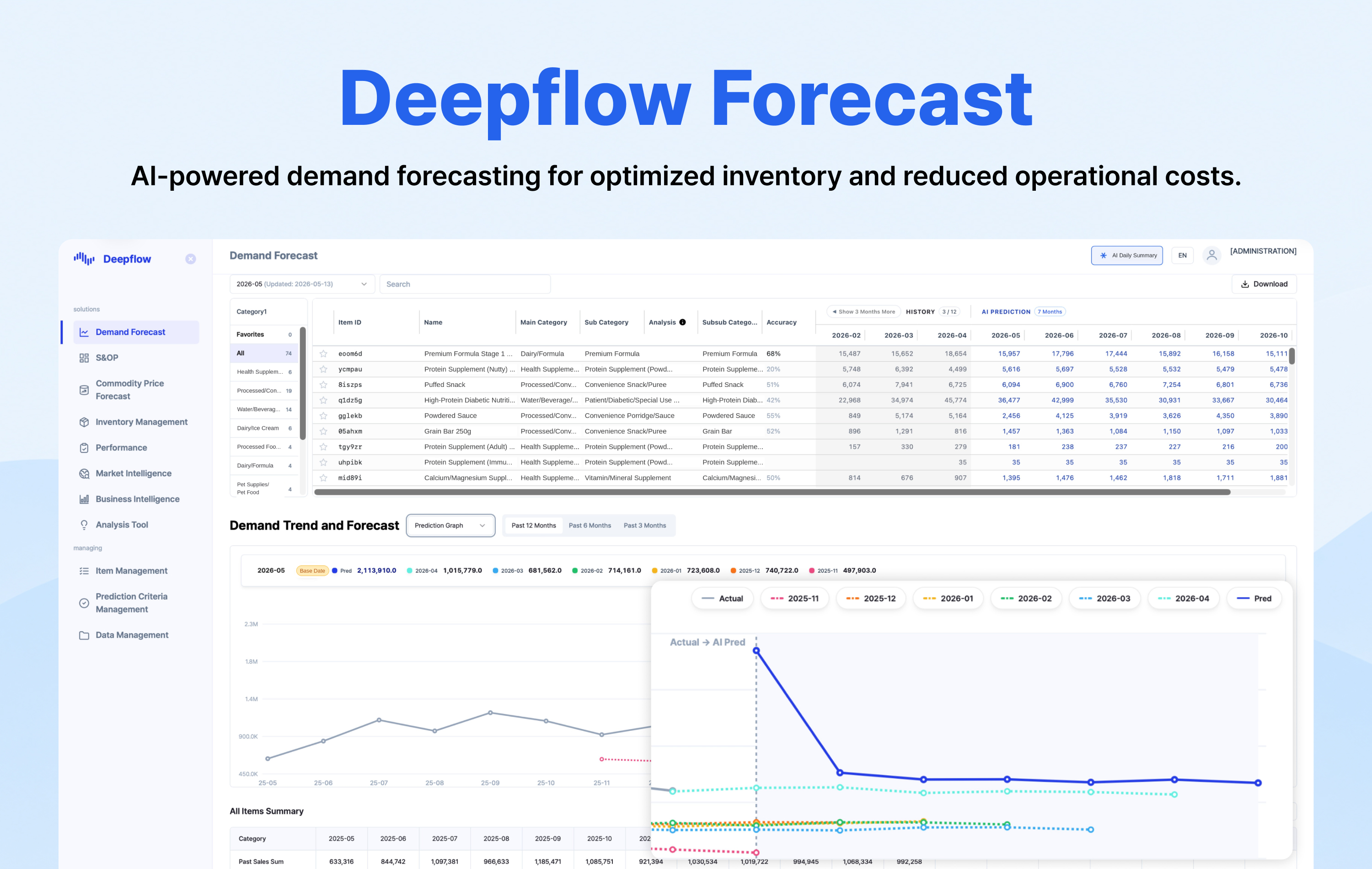
These reviews should not end once the model has been built. During ongoing operations, it remains necessary to distinguish periods when stockouts prevented sales from periods when demand genuinely declined, and to record the reasons behind temporary sales increases. It is also important to check whether forecasts consistently overestimate or underestimate sales for particular products.

Deepflow Forecast’s sales anomaly management feature allows users to record causes such as stockouts, promotions, and one-time external events. This context helps inform subsequent forecast reviews and provides a basis for refining future training data.

If forecasts repeatedly miss the mark for specific products or promotional periods, review what information is incorporated into training and how the results are evaluated. If you are unsure where to begin, explore your available data and opportunities for improvement with us through a free Deepflow proof of concept (PoC).