.svg)

.svg)
Download Brouchure
%202.svg)
Oops! Something went wrong while submitting the form.

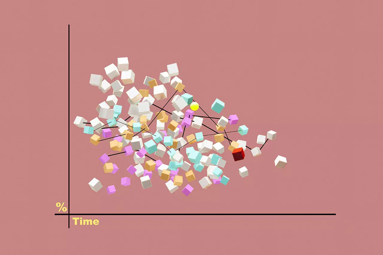
Every demand forecasting professional has wrestled with this puzzle at some point. Why does the forecast hit perfectly for the same product in one month, yet miss by over 30% in another? This forecast variance creates a costly cycle of overstock and stockouts, ultimately eroding trust in business decision-making. This is where external variables become crucial. When you properly incorporate external factors like weather, economic indicators, raw material prices, and consumer sentiment into your forecasting model, you can dramatically reduce forecast variance.
Reducing forecast variance through external variables actually stems from covariate adjustment techniques that statisticians have studied for decades. The core idea is straightforward. You incorporate external factors that correlate highly with your outcome variable to reduce unexplained variation in your model.
Consider forecasting ice cream sales. Looking solely at historical sales patterns shows wide fluctuations. However, when you add temperature data, you can explain a substantial portion of sales variation through temperature alone, which reduces the remaining uncertainty. By explaining predictable variation with external variables, you decrease your model's variance and achieve more accurate forecasts with the same data.
This approach becomes even more critical in demand forecasting. A manufacturer's raw material demand responds to finished goods market conditions, competitor trends, and exchange rate fluctuations. A retailer's product sales connect with weather, economic indicators, and online trends. Systematically incorporating these external variables into your model forms the foundation of improved forecasting power.

Methods for using external variables in practice range from simple to highly sophisticated. Each technique has advantages and limitations depending on your data characteristics and business situation, so choosing appropriately matters.
The most fundamental method is multivariate regression adjustment. When forecasting demand, you build a regression model that includes not just historical sales but also variables like weather, promotion status, and economic indicators. Many companies choose this as their first step because implementation is simple and interpretation is straightforward.
This works particularly well when relationships between variables are relatively linear. For example, if air conditioner sales increase proportionally with rising temperatures, simply adding temperature as a variable to your regression equation produces noticeably better forecast accuracy. However, it struggles to capture complex nonlinear relationships or interactions between variables.
A more advanced form is the CUPED technique. This method, developed by Microsoft in 2013, uses data from the same period in the past to adjust current forecasts. For instance, you reference last year's sales for the same month to calibrate this year's forecast.
While simple enough to implement in SQL, it effectively reduces variance for product categories with strong seasonality. In fact, if the correlation coefficient between last year's data and this year's forecast is 0.7, you can reduce variance by roughly 50%. This proves especially useful in industries with distinct seasonal patterns like apparel, food and beverage, and consumer electronics. However, because it uses only a single covariate, it has limited explanatory power in complex business environments.
When you need higher accuracy, the CUPAC method deserves consideration. This extends CUPED using machine learning models. It simultaneously examines multiple external variables and discovers nonlinear relationships.
For example, models like LightGBM or XGBoost can learn from weather, promotions, competitor pricing, and social media mentions all at once to identify complex patterns. Delivery platform companies have used this method to significantly improve delivery time predictions. DoorDash applied this technique to detect smaller effects, which accelerated their experimentation velocity. However, model training takes time, and you need to be careful not to accidentally include variables affected by the treatment process, which can introduce bias.
The most sophisticated approach is Doubly Robust estimation. It combines two models to create a dual protection effect. One model captures how external variables affect demand, while the other predicts demand itself.
This robust method delivers accurate estimates as long as either model works correctly. It produces the most efficient estimates when you need to identify heterogeneous effects, such as when external variables impact products differently or when promotion effects vary across customer segments. European delivery platform Glovo applied this technique to recommendation algorithm testing and shortened experiment duration by 30% while improving forecast accuracy by 40%. However, implementation is complex and computationally intensive, so you should approach it carefully when dealing with large-scale SKU environments.
ImpactivAI's Deepflow, a leading platform from a demand forecasting specialist company, has built specialized capabilities in this field by automating the use of external variables.
Deepflow's core strength lies in AutoML-based process automation. Without users manually selecting variables or tuning models, the system automatically identifies the optimal feature combination from 500 million possibilities. Various algorithms compete, from cutting-edge transformer-based time series models like I-transformer and TFT to GRU, DilatedRNN, TCN, and LSTM, selecting the best-fitting model for each SKU.
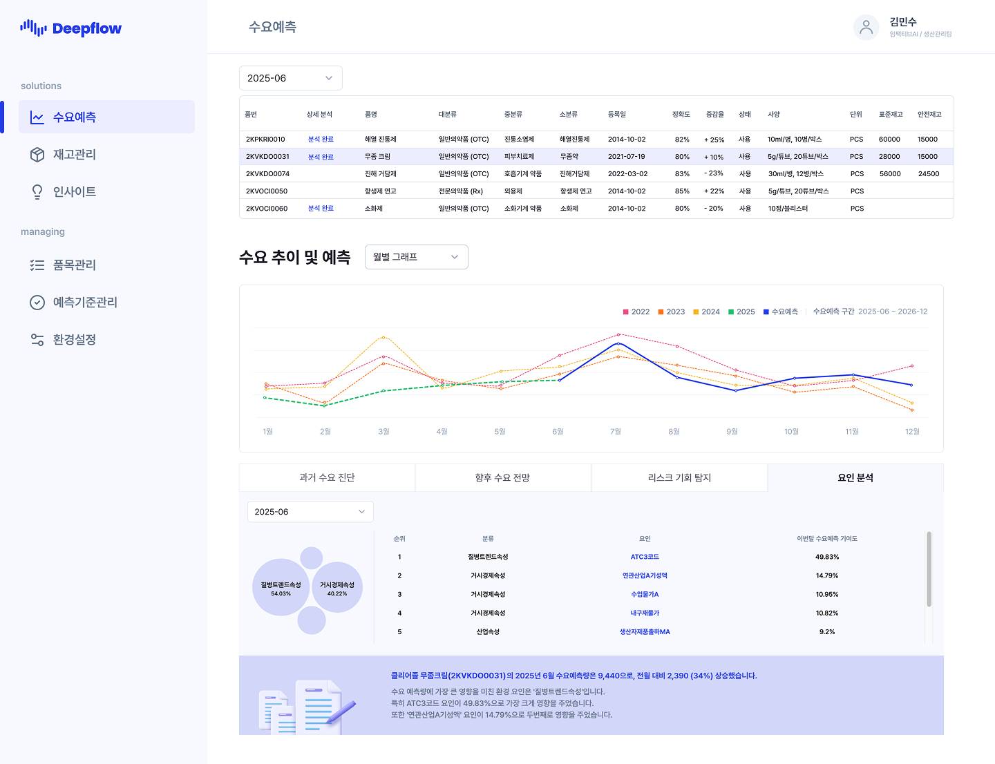
Going beyond simply presenting forecast results, Deepflow specifically explains which external variables influenced the forecast. Through LLM-based insight reports, it articulates forecast reasoning in natural language, such as "this month's demand increase primarily stems from raw material price increases and exchange rate fluctuations," providing explanations that practitioners can immediately understand.
This explainability plays a pivotal role in actual decision-making processes like S&OP meetings and inventory adjustments. Practitioners can communicate with management based on logical reasoning that "these results emerged from specific variable influences" rather than simply stating "AI forecasted this."
Deepflow Material specifically analyzes relationships between external economic indicators and variables for raw material price forecasting using AI. Applied to diverse items from metals like copper and aluminum to agricultural and marine products and construction materials, it has recorded forecast accuracy up to 98.6%. This results from the model automatically learning and incorporating complex external variables like exchange rates, international market conditions, and inventory levels.
Companies that implemented Deepflow experienced an average 33.4% reduction in inventory excess and shortage, with one client cutting inventory costs by 24.8 billion won per month. This stems not simply from superior algorithms but from infrastructure that systematically converts external variables into data and automatically incorporates them into models.
External variables aren't a silver bullet. You need to avoid several practical pitfalls. The most common mistake is indiscriminately adding variables with unclear causal relationships. A variable used in forecasting might actually be a consequence of demand. For instance, if you include discount rate as an external variable but actually offer more discounts when demand is low, the causal relationship becomes reversed.
Adding too many variables also risks overfitting. While accuracy appears high on training data, performance on actual forecasts can actually decline. Cross-validation to confirm actual forecasting power becomes essential.
Variable selection follows principles. Variables must be measurable before demand occurs, show clear correlation with demand, and provide continuously available data. One-time event data, regardless of how impactful, lacks reproducibility and proves difficult to incorporate into models.
Technique selection also varies by situation. When you have sufficient data and complex relationships, advanced techniques like CUPAC or Doubly Robust offer advantages. Conversely, when data is limited or rapid implementation is needed, simpler methods like multivariate regression or CUPED prove more practical. What matters isn't using the most complex technique unconditionally but choosing based on your data and business situation.
Reducing forecast variance using external variables represents a core strategy for elevating demand forecasting accuracy to the next level. Moving beyond simply looking at historical patterns to systematically incorporating various external factors affecting demand enables stable and trustworthy forecasts. When you select techniques appropriate for your business situation and continuously validate and improve them, you'll achieve tangible results in inventory optimization and decision-making quality improvement.
.svg)

.svg)